Introduction

I recently bought a new car with automatic transmission (I’m from EU and they aren’t very common here) and adaptive cruise control. I was blown away when I didn’t have to use gas or brakes if there was a car in front of me. Also while my hype lasted I spent a lot of time looking at other even fancier cars with lane assist and other assist systems. So just for the fun of it I decided to try implementing a simple proof-of-concept algorithm that would detect lanes on a road. Let’s do it!

I recorded some sample footage while driving on the highway and decided to go from there. After we’re done with this post here’s what we’re gonna build:

For the lazy: all of the source code is available at https://github.com/JanHalozan/LaneDetector.

Prerequisites

For starters it’s nice to have OpenCV installed. OpenCV is a beast when it comes to processing images. It’s what allows dummies like me to actually make something :) If you’re struggling with getting it to work here’s an installation that worked for me (OS X).

Second thing is basic knowledge of OpenCV functions. If you don’t know what a cv::Mat is I recommend doing a simple CV tutorial first and then coming back.

Now that that’s out of the way let’s get cracking!

The algorithm

Before we get our hands dirty let’s think a bit how one might approach this problem. All of the code will be in the next section.

Detecting curved lines is quite hard from the camera’s point of view. If we could get a bird’s eye view of the scene it would make things easier as we’d be looking for straight line segments. Oh wait.. we can!

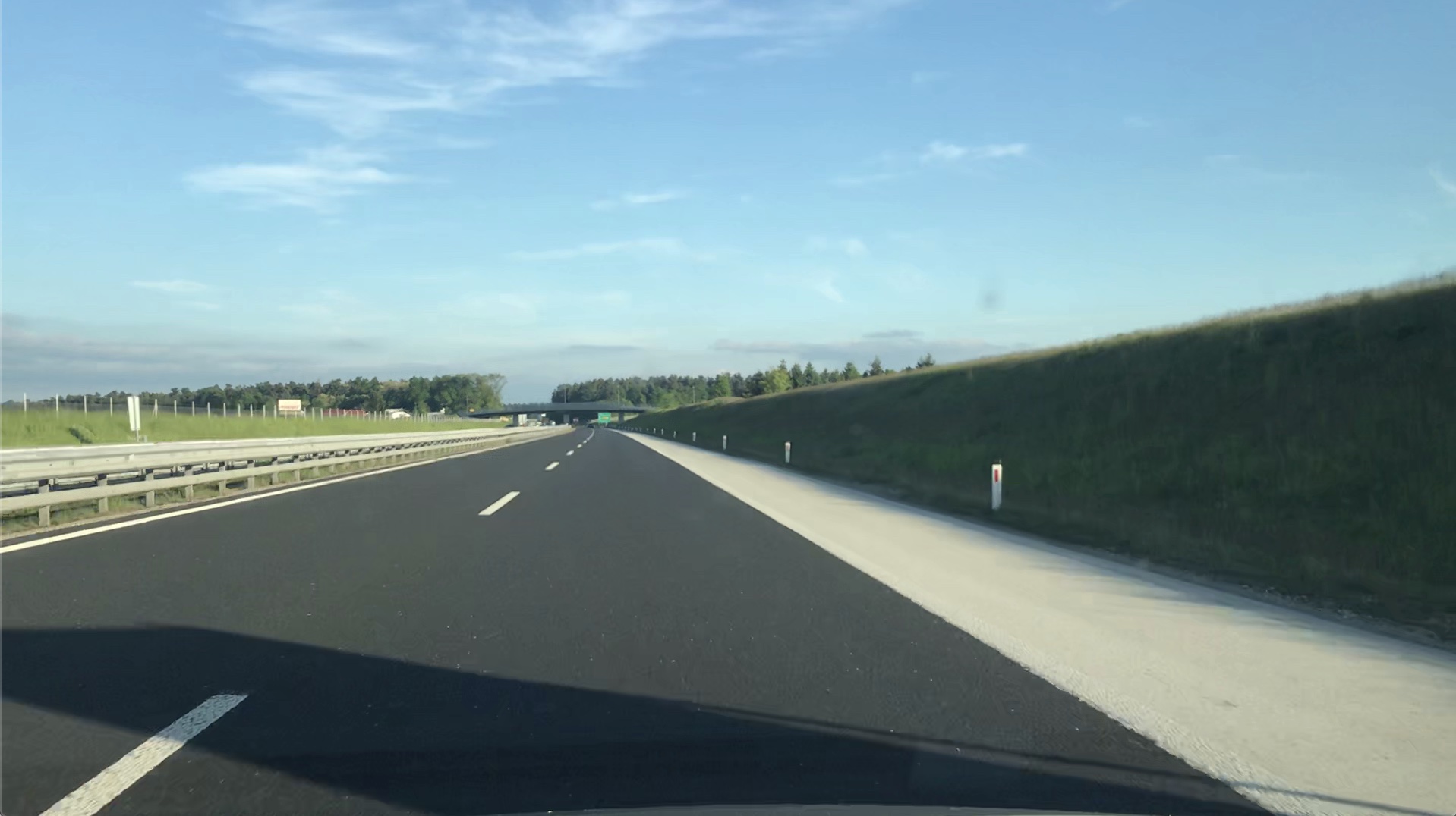
First we’ll transform the image into a bird’s eye view of the scene which we’ll then process to extract the necessary info. We’ll do that by using perspective transformations. We’ll use the top down image for all our detection and once we have all the data we need we’ll transform it back into camera’s point of view. Here’s how the initial image looks like:

And then the converted top down version. We do not convert the entire image but just the region that interests us.

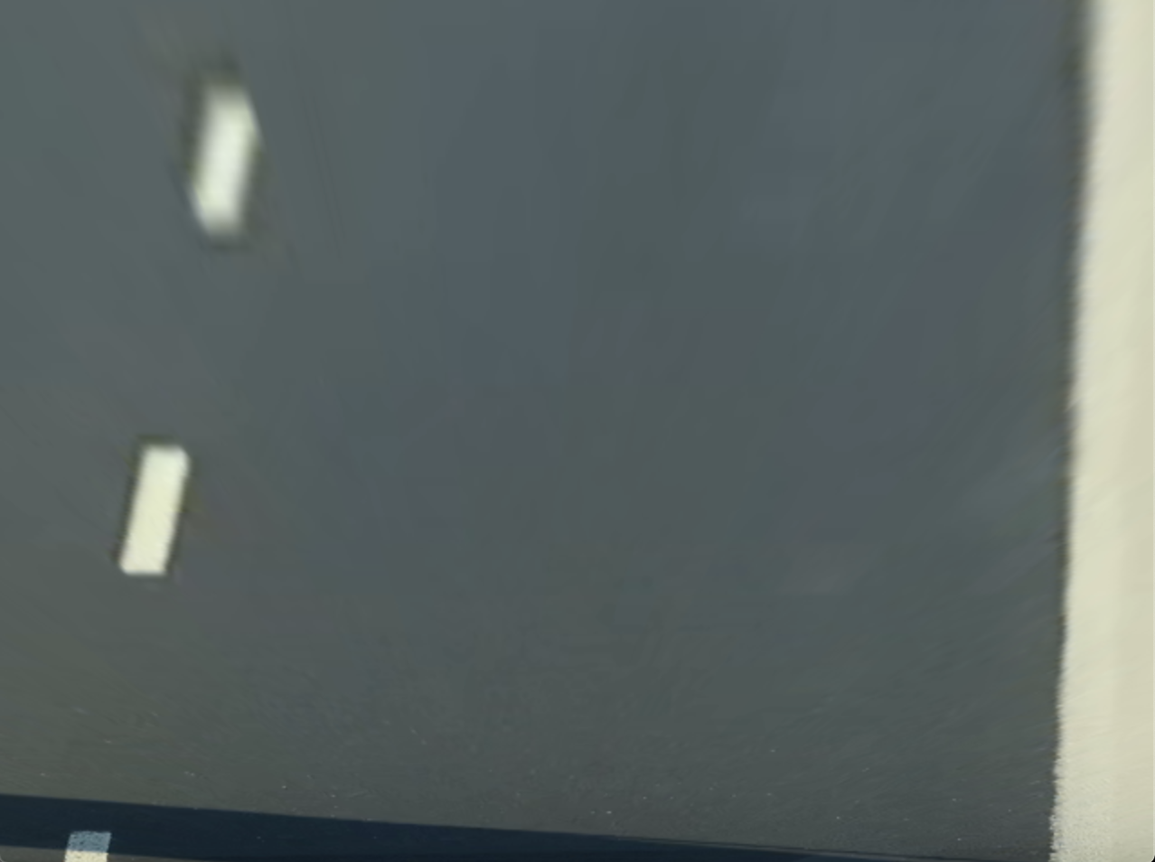
While it’s not your top of the line 4k quality it does allow us to extract all the information we need. What we’re interested in are the lines. We can extract that data by filtering using colors. So we’ll try to extract only white and yellow data from the image. That should ignore most of the surroundings. This is how this step looks like:

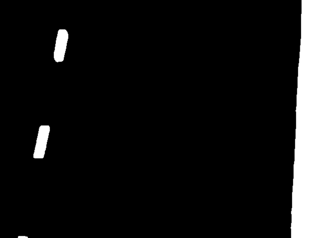
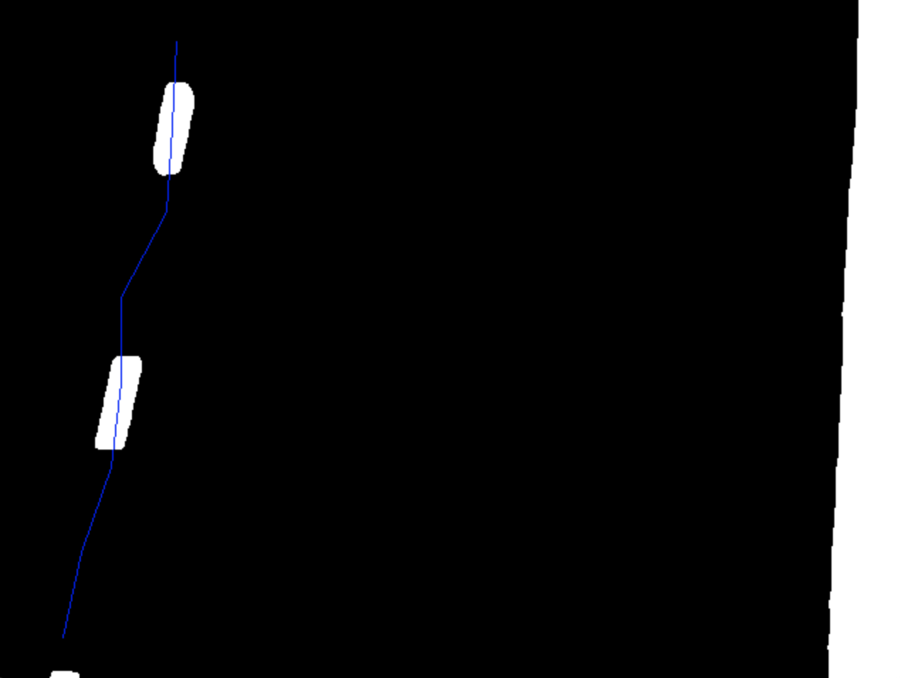
Then some image processing magic will make sure that noise and gaps are removed. If you look at the bottom right corner of the above image you can see some noise and pixels. The exact techniques used in this step can be seen in the code in the next section. We will then also use a simple thresholding function that will convert everything (presumably) useful to white and the rest to black. We get an image like this:

The rest hast to do with extracting the lines data from the white pixels. For that I used a simple sliding window algorithm which will give us the points that we’ll use to mark the lanes. How the algorithm works will be explained in the next section with the actual code. After we have the points we can connect them to get a simple lane.

We can then transform the points back into the camera’s space and visualise them yielding the final result:

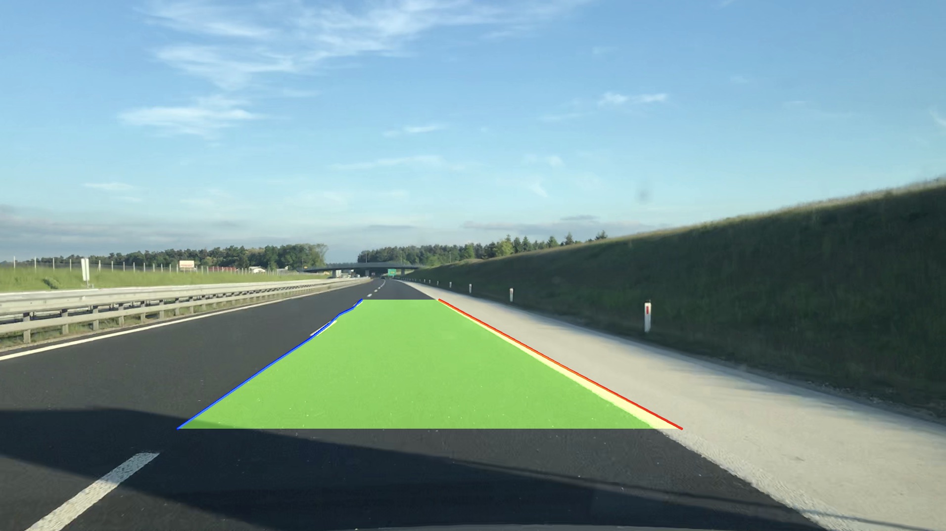
The image above had the sliding window applied on both lanes whereas the image before that had just the left lane for demonstration purposes.

How do we code this in C++ you might ask?

Show me the code!

With respect to the algoritm described above we have to start first by reading the video file. This is just regular OpenCV boilerplate.

Mat org;
    
while (true)
{
    cap.read(org); //Read a frame
    if (org.empty()) //When this happens we've reached the end
        break;

    imshow("Result", org); //Show the image

    if (waitKey(50) > 0) //Wait if a key is pressed then exit otherwise run the loop again
        break;
}

cap.release(); //Don't forget to clean up after ourselves

So we read the image frame by frame and display it. The algorithm described above is pretty simple and works on a single image instead of a sequence. So what we’ll do is we’ll read the image frame by frame like above and run each frame through the algoritm. Let’s start by preparing a bird’s eye view.

Code:

Point2f srcVertices[4];
    
//Define points that are used for generating bird's eye view. This was done by trial and error. Best to prepare sliders and configure for each use case.
srcVertices[0] = Point(700, 605);
srcVertices[1] = Point(890, 605);
srcVertices[2] = Point(1760, 1030);
srcVertices[3] = Point(20, 1030);

//Destination vertices. Output is 640 by 480px
Point2f dstVertices[4];
dstVertices[0] = Point(0, 0);
dstVertices[1] = Point(640, 0);
dstVertices[2] = Point(640, 480);
dstVertices[3] = Point(0, 480);

//Prepare matrix for transform and get the warped image
Mat perspectiveMatrix = getPerspectiveTransform(srcVertices, dstVertices);
Mat dst(480, 640, CV_8UC3); //Destination for warped image

//For transforming back into original image space
Mat invertedPerspectiveMatrix;
invert(perspectiveMatrix, invertedPerspectiveMatrix);

So first we define the region of interest (in pixels) on our original image. The values in srcVertices are what (more or less) worked for me. This is a matter of trial and error and is easiest done by having sliders for tweaking the values. Note that the orientation of points is important and must be kept same for both srcVertices and dstVertices. So our output image will be 640 by 480 pixels which is enough to extract the information we need. Then we call getPerspectiveTransform which provides us with the transformation matrix. We also prepare an inverted transformation matrix which we’ll use to transform points that we find on the bird’s eye image back into the original image. More on that can be found here.

After we have the transformation matrix we can use it to obtain a bird’s eye frame:

warpPerspective(org, dst, perspectiveMatrix, dst.size(), INTER_LINEAR, BORDER_CONSTANT);

This will yield the first step of the algorithm. Next thing we’ll do is convert the image to grayscale as it will make the processing easier. It’s usually easier to extract information from a single channel than multiple.

//Convert to gray
cvtColor(dst, img, COLOR_RGB2GRAY);

//Extract yellow and white info
Mat maskYellow, maskWhite;

inRange(img, Scalar(20, 100, 100), Scalar(30, 255, 255), maskYellow);
inRange(img, Scalar(150, 150, 150), Scalar(255, 255, 255), maskWhite);

Mat mask, processed;
bitwise_or(maskYellow, maskWhite, mask); //Combine the two masks
bitwise_and(img, mask, processed); //Extract what matches

As mentioned we convert the image to greyscale first. Then we create a mask image which contains presumably yellow and white pixels in our greyscale image. That’s what inRange function does. Whatever lies between Scalar(150, 150, 150) which is a very light gray and Scalar(255, 255, 255) which is white is added to maskWhite in this case. Same is done for yellow-ish colours. We then combine the two masks (bitwise_or) into a single one (named mask) and finally apply it to our image. That way we’re left with white and yellow colours (in greyscale of course) which should be fairly close to what we’re looking for. This is the image #2 of the algorithm.

After that some patching up of the image is done in order to reduce noise, remove gaps, …

//Blur the image a bit so that gaps are smoother
const Size kernelSize = Size(9, 9);
GaussianBlur(processed, processed, kernelSize, 0);

//Try to fill the gaps
Mat kernel = Mat::ones(15, 15, CV_8U);
dilate(processed, processed, kernel);
erode(processed, processed, kernel);
morphologyEx(processed, processed, MORPH_CLOSE, kernel);

For that we use some simple gaussian blurring and erosion and dilation. If needed we could use multiple iterations of this step.
To understand in detail what this does I’d recommend looking up the documentation for each of the functions. Some examples can be found here.

Now all we need to do is threshold the image so that what’s interesting is a solid white and rest is black and deemed useless.

//Keep only what's above 150 value, other is then black
const int thresholdVal = 150;
threshold(processed, processed, thresholdVal, 255, THRESH_BINARY);

This produces image #3.

And now we’re finally ready to start the sliding window part of the algorithm. The call looks as follows:

vector<Point2f> pts = slidingWindow(processed, Rect(0, 420, 120, 60));

First argument is a Mat image and second is the starting Rect for the algorithm. Here’s the implementation:

vector<Point2f> slidingWindow(Mat image, Rect window)
{
    vector<Point2f> points;
    const Size imgSize = image.size();
    bool shouldBreak = false;
    
    while (true)
    {
        float currentX = window.x + window.width * 0.5f;
        
        Mat roi = image(window); //Extract region of interest
        vector<Point2f> locations;
        
        findNonZero(roi, locations); //Get all non-black pixels. All are white in our case
        
        float avgX = 0.0f;
        
        for (int i = 0; i < locations.size(); ++i) //Calculate average X position
        {
            float x = locations[i].x;
            avgX += window.x + x;
        }
        
        avgX = locations.empty() ? currentX : avgX / locations.size();
        
        Point point(avgX, window.y + window.height * 0.5f);
        points.push_back(point);
        
        //Move the window up
        window.y -= window.height;
        
        //For the uppermost position
        if (window.y < 0)
        {
            window.y = 0;
            shouldBreak = true;
        }
        
        //Move x position
        window.x += (point.x - currentX);
        
        //Make sure the window doesn't overflow, we get an error if we try to get data outside the matrix
        if (window.x < 0)
            window.x = 0;
        if (window.x + window.width >= imgSize.width)
            window.x = imgSize.width - window.width - 1;
        
        if (shouldBreak)
            break;
    }
    
    return points;
}

What we do is essentially:

Extract a subregion defined by the Rect of the image
Locate all non-zero pixels (which are all white in our case)
Calculate the average X position of those pixels
(optional) if there are none use the same X that was used in this iteration
Iterate until we reach the top of the image

Each average X position is used as a point while Y is supplied from moving the window up by its height on each iteration. Visually it looks like this:

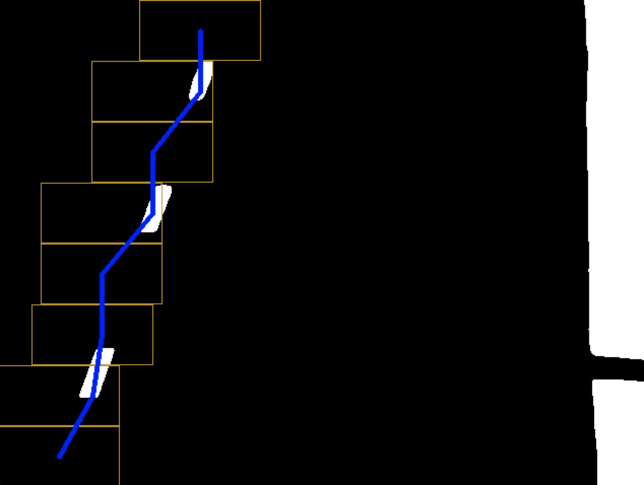
You can see how the first region of interest (ROI) had no white pixels so the window just moved up. The next ROI had pixels right of its center so the next window moves right and so on.

It’s worth noting that the calls in the code provided use hardcoded rects (bottom left for left lane and bottom right for right lane) which can cause some problems. It would be better to calculate a histogram with respect to the x axis and use the two highest values as starting x positions for the window.

Once we have the points it’s just a matter of visualizing them on the initial image.

vector<Point2f> pts = slidingWindow(processed, Rect(0, 420, 120, 60));
vector<Point> allPts; //Used for the end polygon at the end.

vector<Point2f> outPts;
perspectiveTransform(pts, outPts, invertedPerspectiveMatrix); //Transform points back into original image space

//Draw the points onto the out image
for (int i = 0; i < outPts.size() - 1; ++i)
{
    line(org, outPts[i], outPts[i + 1], Scalar(255, 0, 0), 3);
    allPts.push_back(Point(outPts[i].x, outPts[i].y));
}

allPts.push_back(Point(outPts[outPts.size() - 1].x, outPts[outPts.size() - 1].y));

Mat out;
cvtColor(processed, out, COLOR_GRAY2BGR); //Conver the processing image to color so that we can visualise the lines

for (int i = 0; i < pts.size() - 1; ++i) //Draw a line on the processed image
    line(out, pts[i], pts[i + 1], Scalar(255, 0, 0));

//Sliding window for the right side
pts = slidingWindow(processed, Rect(520, 420, 120, 60));
perspectiveTransform(pts, outPts, invertedPerspectiveMatrix);

//Draw the other lane and append points
for (int i = 0; i < outPts.size() - 1; ++i)
{
    line(org, outPts[i], outPts[i + 1], Scalar(0, 0, 255), 3);
    allPts.push_back(Point(outPts[outPts.size() - i - 1].x, outPts[outPts.size() - i - 1].y));
}

allPts.push_back(Point(outPts[0].x - (outPts.size() - 1) , outPts[0].y));

for (int i = 0; i < pts.size() - 1; ++i)
    line(out, pts[i], pts[i + 1], Scalar(0, 0, 255));

//Create a green-ish overlay
vector<vector<Point>> arr;
arr.push_back(allPts);
Mat overlay = Mat::zeros(org.size(), org.type());
fillPoly(overlay, arr, Scalar(0, 255, 100));
addWeighted(org, 1, overlay, 0.5, 0, org); //Overlay it

imshow("Output", org);

In the code above we use the sliding window first and then we use perspectiveTransform with the invertedPerspectiveMatrix to transform points from the bird’s eye view into camera’s view. Rest is drawing lines on the top down image and the final output image and finally we use the fillPoly and addWeighted to draw a green overlay for our lane.

This gives us the final result. Nice!

Conclusion

Without too much hassle we implemented a simple lane detecting algorithm from scratch. It’s not the most robust of the lot but it demonstrates a possible way to approaching the problem. It can be made more resilient with better preprocessing and improved left / right lane sliding window (for example on left lane we should lean a bit more towards right instead of actual average, …).

Fitting a polynomial (ie. curved lanes)

Right now we get a polygon of straight line segments. It would be nicer if we could fit a polynomial curve that would show the actual curvature of the lanes. If the language of implementation was Python we could easily use Numpy which has built in functionality for such tasks. In C++ we’d have to roll our own which I might do some day. For now you can refer to this example of how to do it. It uses the least squares fitting method and should work just fine.

Future work

Another cool thing would be to add an AI library and perhaps detect other cars on the road or road signs. Again it’s something I might do in the future. If you want to approach this I’d recommend TensorFlow’s object recognition library.

An OpenCV Lane Detector for dummies in C++

Let's see if we can build a simple lane detecting algorithm.